First Simulation
This Tutorial aims to enable the user to start the first simulation with DINO. The user gets familiar with the following steps:
- creating an input file for a simple simualtion set-up from scratch
- running DINO
- description and simple post-processing of output-data
The auto-ignition of a hydrogen–air mixture is used as an example. This case requires only limited computational resources and can be performed with a single processor. At the same time, it illustrates the key working steps as well as the main inputs and outputs of DINO.
The auto-igniton refers to the spontaneous initiation of combustion in a reactive mixture without an external ignition source such as a spark or flame. It occurs when the mixture reaches a critical temperature and pressure at which chemical reactions accelerate rapidly. This acceleration leads to a sudden release of heat, causing the mixture to ignite on its own. The time required for the acceleration of chemical reactions until combustion begins is referred to as the ignition-delay time. It represents an important parameter for validating kinetic models, for example in simulations of engine processes. In our first simulation we want to try to observe the ignition-delay-time of the auto-ignition of Hydrogen in Air.
Therefor a quasi-one-dimensional domain with dimensions of 8.5 mm × 8.5 mm × 0.12 mm is defined for the simulation. One node is applied in the y- and z-directions, while eight nodes are used in the x-direction. Periodic boundary conditions enclose the domain. Inside the domain, a stoichiometric mixture for hydrogen combustion in air is specified. Based on the reaction equation
the mixture composition results in mole fractions of 1 for H₂, 0.5 for O₂, and 1.88 for N₂.To trigger auto-ignition an initial high temperature of 1750.5K at normal pressure 101325Pa is needed. Lets have a look if we can determine the correct ignition-delay-time!
Creating run directory
All your future DINO projects should be placed in a seperate folder: the run directory. We suggest you to create run directory outside the DINO directory tree and run your cases there. You can also create several different run directories according to different projects. For your first simulation go to your home directory and create the direcory dino_runs.
dino_runs directory.
For Sofja users at OvGU
For the Sofja cluster you should creat this directories in /scratch
Creating your own DINO_IN file from scratch
Every simulation carried out with DINO requires an input file named DINO_IN. This file contains all necessary parameters for performing a DINO simulation. The parameters are organized into Fortran namelist sections. Each section includes several input variables together with their assigned values. For example, the variable INIT_TEMPERATURE appears in the section INITIALIZE and specifies the initial temperature of the computational domain.
Hint
See all namelist sections and there corresponding parameters in the descripton of main-input-file.
For the first Simulation you can create your own DINO_IN file from scratch. Therefore open a new text-file in the first_simulation directory with the text editor of your choice (here we use vim).
DIMENSIONS section is used. The following lines create the corresponding namelist section and specify the required variables for the domain size:
    &NML_DIMENSIONS
        LENGTH_X=0.12D-3,
        LENGTH_Y=8.5D-3,
        LENGTH_Z=8.5D-3,
        DIMX_TOTAL=8,
        DIMY_TOTAL=1,
        DIMZ_TOTAL=1,
    /
The number of grid points in the Cartesian grid is controlled by DIMX_TOTAL, DIMY_TOTAL, and DIMZ_TOTAL. In the x-direction, 8 nodes are used, while in the y- and z-directions only one node is applied. This creates a quasi-1D domain with the correct dimensions.
Next, the grid generation must be defined. For this purpose, the GRIDDING namelist is created, and DINO is instructed to generate an equidistant Cartesian grid in all directions by setting the variable GRID_TYPE to 1:
For your domain you should also define the boundary conditions. For that reason create the namelist section BOUNDARY and define the left, right, top, front and back boundary as periodic. Note that the boundary variables only accept integer as values. The periodic boundary condition corresponts to the value 3.
Hint
For defining other boundary conditions use different values between 0 and 10. The corresponding boundary conditions to the values are descibed here.
In the next step we define the time-step control parameters and the time integration sheme. Creat the namelist CONTROL and TIME_INTEGRATION and define an initial time step of \(1 \cdot 10^{-8}\)s, a minimum time step of \(1 \cdot 10^{-10}\)s and a maximum time step of \(1 \cdot 10^{-7}\)s with 4th order explicit runge-kutter integration sheme. You should also define here the end time of the simulation with \(1.2 \cdot 10^{-4}\)s.
    &NML_CONTROL
        INIT_TIMESTEP=1.0D-8,
        TSTEP_MIN=1.0D-10,
        TSTEP_MAX=1.D-7,
        TIME_END=1.2D-4,
    /

    &NML_TIME_INTEGRATION
        INTEGRATION_SCHEME=1,
    /
Hint
INTEGRATION_SCHEME only accept integers as input values. Use value between 1 and 5 for different time integration schemes. Find the description of differen values here.
Now you created the domain with boundary conditions and the time-step control. What is missing are the definition of the initial conditions and the reactions taking place with the ignition of H2 in Air. Therefor create the namelist INITIALIZE and define the initial pressure with 101325 Pa and the inital temperature with 1075.5 K. For defining the mechanism of reactions a cantera input file is used. You can create your own cantera input file and define mechanisms as described in the documentation of cantera. For this tutorial we use a already defined and well known mechanism for the combustion of H2 in Air from Williams. The mechanism is described in the cantera input file h2_williams_12.xml under WORK/MECHANISMS/h2_williams_12. For using the predefined mechanism we just add the name of the mechanism as value for the variable GAS_PHASE(1). You should also provide an initial compositon of the gas mixture in mole frations. In our case we have perfect stoichometric conditions for the combustion of H2 in Air which relates to the mole fractions of 1 for H2, 0.5 of O2 and 1.88 of N2 as seen at the bigging of this tutorial in the reaction equation. Dont worry about the fact that mole fractions are together in sum greater than one, Cantera and DINO will normalize it for you.
    &NML_INITIALIZE
        INIT_PRESSURE=101325.D0,
        INIT_TEMPERATURE=1075.5D0,
        GAS_PHASE(1)='h2_williams_12',
        GAS_PHASE(2)='H2:1.0, O2:0.5, N2:1.88',
    /
REACTION is required. Here you define if the simulation is reactive with variable REACTIVE=.true. and define the start of the reaction and the method used for calculating the physico-chemical modell. Here we use PHYSCHEM_LIB=1 which corresponds to Cantera as method.
For the rest of the parameters which are not required you dont need to mention them in your DINO_IN file. The only step which is necessery is tomention all the rest of the required namelists as described below:
&NML_IMMERSED_BOUNDARY
    IB_NUMBER=1,
/

&NML_DECOMPOSITION
/

&NML_POISSON_SOLVER
/

&NML_RESTART
/

&NML_RADIATION
/

&NML_POD
/

&NML_TRANSPORT
/

&NML_GRAVITY
/

&NML_VORTEX
/

&NML_TWOPHASE
/

&NML_TURBULENCE
/

&NML_NANOPARTICLES
/
DINO_IN file has all required informations for running your first simulation. But before running you should decide which kind of output is needed. Therefor you should take a closer look at the namelist SAVING.
    &NML_SAVING
        SAVING_TYPE=1,
        SAVING_RESTART_INTERVAL=1500,
        SAVING_AVERAGE_INTERVAL=10000,
        SAVING_CTRL_MAX_MIN_INTERVAL=50,
        SAVING_HDF5_FULL=.true.,
        SAVING_CTRL_HDF5_INTERVAL=500,
        SAVING_HDF5_START=0,
    /
SAVING_TYPE determines whether to save result based on time (SAVING_TYPE=0) or iteration steps (SAVING_TYPE=1). In the Case your Simulation is breaking up for any reason the SAVING_RESTART_INTERVAL is a helpful variable. It determines the interval between saving restart files. With these files you can restart your simulation from the last point of iteration, where a restart file was created. The SAVING_AVERAGE_INTERVAL determines the number of iterations for data accumulation before averaging. The SAVING_CTRL_MAX_MIN_INTERVAL determines the number of iterations between saving ASCII data files storing maximum and minimum values of different variables. the rest of the variables a meant to controll the HDF5 output. You can enable HDF5 output, set up the starting iteration for saving HDF5 files and determine the interval between savings.
Running DINO
Now your simulation is ready to run. To launch the calculation, go to your project folder first_simulation and run the executable file DINO_V<version>.e. The executable
file will use DINO_IN in the current directory as the default input file. If a different input file
should be used, the path to that file can be given as the first command line argument to the DINO
executable.
If the case is to be run on a supercomputer or cluster, a job command file can be created and used, depending on the server/machine where the simulation is to be performed. For more information about these scripts, you should contact your institute/company/HPC help desk.
For Sofja users at OvGU
You can use the following procedure to run the simulation with Slurm job manager on Sofja.
Copie the following lines into yourlaunch_script.sh:
    #!/bin/bash
#SBATCH -J DINOfirstsim
#SBATCH -N 1
#SBATCH --ntasks-per-node 1
#SBATCH --cpus-per-task=1
##SBATCH --cpu-bind=threads
##SBATCH -d singleton
#SBATCH --time 00:10:00
#SBATCH --mem 256000
#SBATCH -p  short
##WORKINGDIRECTORY="/beegfs2/scratch/<user>/dino_runs/first_simulation"
module purge
module load mpi/openmpi-4.1
source /beegfs1/software/DINO/env
mpirun -n $SLURM_NTASKS  /beegfs1/software/DINO/dino/bin/dino_v10.0.0_beta.e
launch_script.sh and run DINO with following command:
Output and first post-processing
After you started your first simulation, it will finish very quickly after some seconds due to the TIME_END is reached. Now you can look into your project directory if the following output was created:
- follow_on: This file is giving you information concerning the running computation (time step, time step control, processor configuration ...). It is periodically updated during the simulation.
- data_timevol: In this subdirectory, the time evolution of corresponding variables (density, pressure, temperature, heat release, time step, velocity, species mole/mass fractions, turbulence statistics...) are stored in
dino_timev_<variables>.dat. In each data file, the first column represents time, the definition of other columns can be found in$DINO_HOME/SOURCES/SAVE/dino_io_write_time_history.f90. For example, indino_timev_temper.dat, the second column represents the maximum temperature, the third one is the minimum temperature, and the last one represents the average temperature. - data_hdf5: The binary hdf5 data files for the main variables are stored in this subdirectory.These results are used for post-processing and detailed analysis. Every data file
dino_res_*.h5contains the full solution with all details. The number of iteration steps between data files are defined inDINO_INasSAVING_CTRL_HDF5_INTERVAL. The hdf5 data files can be post-processed by most visualization softwares, such as VIsit, Paraview and Tecplot. Also you can use the provided Matlab or Python scripts ($DINO_HOME/TOOLS/readhdf5.mand/or$DINO_HOME/TOOLS/readhdf5.py) to read and analyze the data in the hdf5 files. - data_restart: In this subdirectory, the restart files named
dino_*are stored. The interval steps between the restart files are defined in the input fileDINO_INasSAVING_RESTART_INTERVAL. All the restart files contain the full solution corresponding to the designated variable. The simulations can restart from any of these restart files.
We can now plot the temperature over time using the tiemevolution data data_timevol and a python script:
import numpy as np
import pandas as pd
import matplotlib.pyplot as plt

# This script plots temperature vs time
# from data_timevol/dino_timev_temper.dat file
df = pd.read_csv('data_timevol/dino_timev_temper.dat', delim_whitespace=True, header=None, names=['Time', 'Temperature_min', 'Temperature_max', 'Temperature_mean'])

plt.figure(figsize=(10, 6))
plt.plot(df['Time'], df['Temperature_mean'], label='Temperature vs Time', color='blue')
plt.title('Temperature vs Time')
plt.xlabel('Time (s)')
plt.ylabel('Temperature (K)')
plt.grid()
plt.legend()
plt.savefig('temperature_vs_time.png')
plt.show()
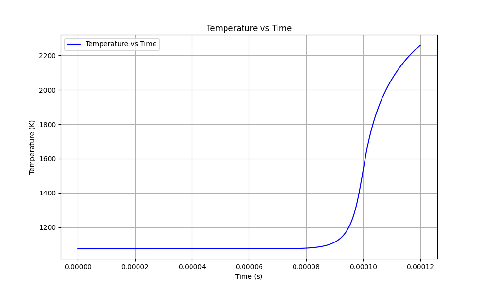 Gases react and get hotter, showing an autoignition iwhere the initial temperature increases by 400 K -- at 0.1 ms of delay time.
We can also plot the massfractions with data_timevol:
import numpy as np
import matplotlib.pyplot as plt
import pandas as pd
from pathlib import Path

data_dir = Path(__file__).resolve().parent / "data_timevol"
file_H2 = data_dir / "dino_timev_y_H2.dat"
file_OH = data_dir / "dino_timev_y_OH.dat"
file_H2O = data_dir / "dino_timev_y_H2O.dat"
file_O2 = data_dir / "dino_timev_y_O2.dat"

try:
    df_H2 = pd.read_csv(file_H2, delim_whitespace=True, header=None,
                        names=['Time', 'MassFraction_H2_min', 'MassFraction_H2_max', 'MassFraction_H2_mean'])
    df_OH = pd.read_csv(file_OH, delim_whitespace=True, header=None,
                        names=['Time', 'MassFraction_OH_min', 'MassFraction_OH_max', 'MassFraction_OH_mean'])
    df_H2O = pd.read_csv(file_H2O, delim_whitespace=True, header=None,
                         names=['Time', 'MassFraction_H2O_min', 'MassFraction_H2O_max', 'MassFraction_H2O_mean'])
    df_O2 = pd.read_csv(file_O2, delim_whitespace=True, header=None,
                        names=['Time', 'MassFraction_O2_min', 'MassFraction_O2_max', 'MassFraction_O2_mean'])
except FileNotFoundError as e:
    raise SystemExit(f"Missing input file: {e.filename}")

def normalize_series(s):
    m = s.max()
    return s / m if m and m > 0 else s * 0.0

y_h2 = normalize_series(df_H2['MassFraction_H2_mean'])
y_oh = normalize_series(df_OH['MassFraction_OH_mean'])
y_h2o = normalize_series(df_H2O['MassFraction_H2O_mean'])
y_o2 = normalize_series(df_O2['MassFraction_O2_mean'])

fig, ax = plt.subplots(figsize=(10, 6))
ax.plot(df_H2['Time'], y_h2, color='tab:blue', label='H2 (normalized)')
ax.plot(df_OH['Time'], y_oh, color='tab:red', label='OH (normalized)')
ax.plot(df_H2O['Time'], y_h2o, color='tab:purple', label='H2O (normalized)')
ax.plot(df_O2['Time'], y_o2, color='tab:green', label='O2 (normalized)')

ax.set_xlabel('Time (s)')
ax.set_ylabel('Normalized mass fraction')
ax.set_ylim(0, 1.05)
ax.grid(True)

# place legend on the left, centered vertically, and expand left margin so it isn't clipped
ax.legend()
fig.subplots_adjust()

plt.title('Normalized species mass fractions vs time')
plt.savefig('mass_fraction_species_normalized_vs_time.png', bbox_inches='tight', dpi=200)
plt.show()
The resulting plot shows you the mass fraction evolution of the most important species:
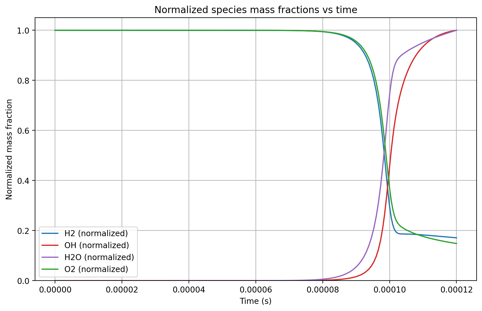
Hydrogen (H2) and oxygen (O2) get consumed, while the hydroxyl (OH) radical as well as water (H2O) molecules are produced.
The ignition delay time can be calculated and compared to reference values with the following post-processing script:
import sys
import numpy as np

# Author: Abouelmagd Abdelsamie
# date:  04.08.2016


mfile= 'data_timevol/dino_timev_temper.dat'
t, tmax= np.loadtxt(mfile, usecols=(0,1), unpack=True)

for i in range(1, len(t)):
    temperature_increase = np.abs( tmax[i] - tmax[0])
    if (temperature_increase >= 400.0):
        current_tau = t[i] * 1000.
        print ('Current auto-ignition delay time = ',round(current_tau,4),' [ms]')
        break

itau= 0.1001 # ms
print ('Reference auto-ignition delay time =',  itau, ' [ms]')

ierror = abs(itau - current_tau)
if (ierror <= 1.e-2):
    print ( 'Auto-ignition delay time test succeeds; Perfect!')
else:
    print ( 'Auto-ignition delay time test fails: there is some thing wrong')
    print ( 'Make sure that you are using Williams kinetic mechanism with 12 species')
--Computing the ignition delay time from DINO
Current auto-ignition delay time =  0.0996  [ms]
Reference auto-ignition delay time = 0.1001  [ms]
Auto-ignition delay time test succeeds; Perfect!
Success
Congratulation! You finished your first simulation with DINO